Category: Nicht kategorisiert

Tl;dnr
The reason for founding the company was to be able to offer a service that I myself would have liked to use more often: to generate complete, gap-filled data series of high quality.



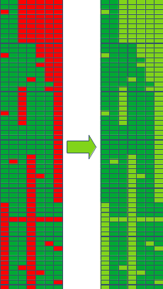
If you want to run a hydrological model, be it a water balance model, a rainfall-runoff model or a flood forecasting model, you need data to drive the model. Runoff cannot be calculated if a year is missing from the precipitation time series. In the vast majority of cases, the data requirements of the model are much higher: the models only run if the input data is available without gaps. Of course, this does not only apply to the models mentioned. Plant growth models, ecosystem modelling, urban climate models and countless others have similar requirements. Measured time series rarely fulfil these requirements: Measurement failures occur for a variety of reasons, or incorrect measurements have to be removed from the data.

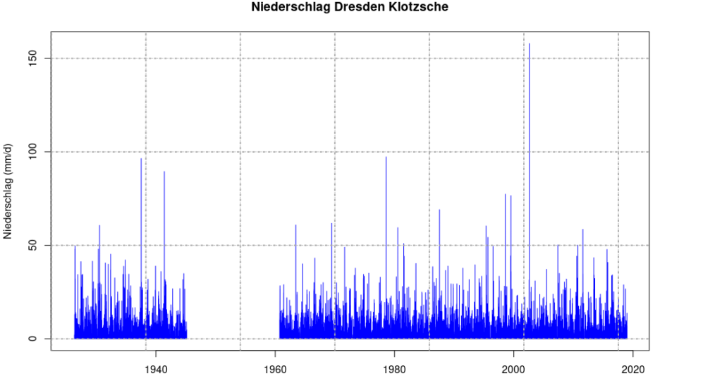
The precipitation station of the German Weather Service in Dresden-Klotzsche, which has no data between 1945 and 1960, is shown here as an example.

In order to obtain complete time series, the nearest station with data is often used in such cases. This leads to inhomogeneous time series, as the neighbouring stations have different statistical properties, such as a different mean value, different extremes and different frequencies of precipitation days. There are other methods, such as spatial interpolation, (multiple) linear regression or the use of reanalysis data, all of which vary in complexity and have their own errors. Whatever you choose, in the end you will have spent a lot of time filling in the gaps or you will have an error-prone time series or, in the worst case, both.

In my own case, I needed hourly values for temperature, wind speed and relative humidity for my work. Compared to daily values, hourly values have three negative characteristics: The time series are shorter, there are significantly fewer time series overall and there are considerably more gaps. In addition, it was particularly important here that the gap-filled data should have as small an error as possible. The aim was therefore not to achieve a reasonably satisfactory result, but to achieve the best possible result. With several hundred time series, each with several hundred thousand time steps, the existing methods proved to be unfeasible. On the one hand, the computing time was exorbitantly high, on the other hand, the quality was insufficient. It was therefore necessary to develop new methods that met both requirements: To realise the smallest possible error in the shortest possible computing time. How and in which areas this was achieved will be explained in the next blog posts.

Filling gaps in time series (for motivation click here) has a lot of methodological requirements:

On the one hand, the quality of the gap filling should of course be high, i.e. the filled values of a time series should be as close as possible to the values that actually occurred but were not measured. This may sound trivial, but there are some simple methods where, for example, the gaps in temperature time series are replaced with annual averages. This preserves the mean value of the time series, but the values at the individual points in time are grossly incorrect.

Next, the methodology should be able to cope with closing the gaps with both a few and many sampling points. Let’s imagine a time series that has been measuring for 20 years and we want to extend it to a length of 100 years (yes, this is possible 🙂). At the beginning of the 20th century, there were only relatively few measuring stations that could be used as reference points. In the last 50 years, however, the number of measuring stations has risen sharply. Now we want to use as much information (i.e. sampling points) as possible for both the distant and more recent past in order to achieve the best possible quality of gap filling.

Now, the time series that are to be used as sampling points to fill the gaps at a particular station also have gaps themselves. This means that the method must be able to deal with gaps in the sampling points. The vast majority of methods cannot do this, so the gaps in the grid points themselves must first be filled using a very simple method, or the number of grid points is drastically reduced. Another option would be to create a separate list of grid points for each gap. All this leads either to a very high calculation time or to greater inaccuracy in the calculation.

Last but not least, the calculation time should of course be tolerable. If you calculate hourly values of meteorological variables for all stations in Germany for several decades, you end up with several hundred thousand time points for several thousand time series. And each of these time series in turn has several hundred time series as supporting points.

The method of choice here is ‘gradient boosting’, or more precisely ‘gradient boosted decision trees’. As the name suggests, decision trees are created here using machine learning methods. These depict the characteristics of the target variable, for example precipitation at a particular station, as a function of various supporting points. These supporting points are precipitation time series from other stations, but other time series such as temperature, humidity, wind speed or the date are also included in the decision trees. The relationship is non-parametric and non-linear; several hundred trees with up to ten levels are used for one image.

The use of gradient boosting already solves some problems: the calculation is extremely fast as it can be performed on graphics cards. Since more time series can be filled in the same time, such a task can of course still take some time. The methodology also makes it possible to use gaps in the sampling points.

Next, gradient boosting should be able to cope with both many and few support points at the same time. This is not always the case; the numerous parameters have to be tweaked in order to achieve this state. We use cross-validation by means of genetic learning for parameter optimisation.

But to be really good, it needs something more. The requirements are manifold: The individual values should be as accurate as possible. The statistics of the entire time series should be preserved. It should be possible to fill short gaps, perhaps only an hour long, as well as to extend a time series by 100 years into the past. For all this, we have developed a framework around the gradient boosting method. This includes state of the art methods such as blending and bagging as well as the clustering of gaps in order to determine sub-periods for gap filling as effectively as possible. Another blog post will soon show what quality can be expected in the various scenarios. An overview of the expected quality for individual gaps can be found here in my 2018 paper.