Filling and extending time series
Brief description
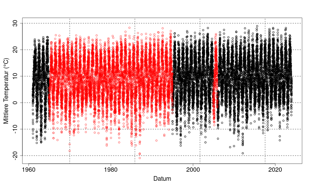
Filling and extending time series is a procedure that aims to close gaps in meteorological measurement series and to extend these series if necessary. The aim is to provide the most complete and continuous data sets possible for various meteorological parameters such as temperature, precipitation or wind speed.
Why fill gaps?
Meteorological measurement series often have gaps, caused by technical failures, maintenance work or other disruptions in measurement operations. Most time series begin after the start of the investigation period or end prematurely. However, for many applications – such as climate analysis, trend determination or modelling – complete time series are necessary. Filling and extending the time series makes it possible to fulfil these requirements and increase the informative value and usability of the data. Complete time series are particularly important as initial data for spatial interpolation: using incomplete time series leads to spatial/temporal breaks in the raster product. If only complete measured time series are used for a raster product, the database is significantly reduced and the quality of the raster data drops sharply.
Procedure
Missing values in existing measurement series are estimated using information from neighbouring stations. Machine learning methods (gradient boosting) are used to minimise the estimation errors.
Quality and properties
We check the quality of the gap filling using independent validation procedures such as cross-validation. This involves temporarily removing known values, reconstructing them using the selected method and comparing them with the original values. The quality of the method can be assessed using statistical indicators such as the mean error or the standard deviation. A high-quality method provides estimates that are as accurate as possible and preserves the statistical properties of the original data.
References
State Institute for the Environment Baden-Württemberg (LUBW):
Climate Atlas Baden-Württemberg, complete daily data for Baden-Württemberg and the surrounding area 1961-2023
State Office for Environment, Agriculture and Geology (LfULG Saxony):
Reference dataset 3.0 in ReKIS, complete daily data for Saxony, Saxony-Anhalt, Thuringia, Brandenburg and surroundings 1961-2023
State enterprise Sachsenforst (SBS):
Gapless daily data of the meteorological data of the forest sites 1961-2023
Literature
Körner, P., Kronenberg, R., Genzel, S., Bernhofer, C., 2018. Introducing Gradient Boosting as a universal gap filling tool for meteorological time series. Meteorologische Zeitschrift 369–376. https://doi.org/10.1127/metz/2018/0908
Creating raster datasets
Description
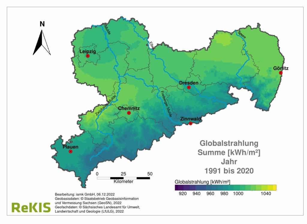
The creation of raster datasets from meteorological station data is a process in which point measurements from weather stations are converted into area-wide, regularly resolved data fields (rasters). These raster datasets represent the spatial distribution of meteorological variables over a specific area.
Why raster data?
Station data only provide punctual information, whereas for many applications – such as hydrological modelling, agricultural planning or climate impact assessment – area-wide information is required. Raster datasets enable analyses and visualisations at regional or national level and are indispensable for linking meteorological data with other geoinformation.
Procedure
Various spatial interpolation methods are used for this purpose, such as kriging or splines. These methods utilise the values of the surrounding stations to calculate a plausible value for each grid cell. This creates continuous fields for parameters such as temperature, precipitation, wind speed or other meteorological variables.
Quality and properties
We check the quality of the generated raster data sets using validation procedures such as cross-validation. This involves excluding individual stations from the interpolation process, calculating the values at these points and comparing them with the actual measured values. The accuracy of the interpolation depends on the station density, the selected method and the spatial variability of the meteorological variable. High-quality raster data sets are characterised by the smallest possible deviations between calculated and measured values and represent the spatial structures of the meteorological variables realistically. For the mean temperature, for example, a coefficient of determination R² of 0.992 and a mean absolute error of 0.52°C are achieved.
References
Baden-Württemberg State Institute for the Environment (LUBW):
Climate Atlas Baden-Württemberg, complete grid data for Baden-Württemberg and the surrounding area 1961-2023
State Office for Environment, Agriculture and Geology (LfULG Saxony):
Reference dataset 3.0 in ReKIS, complete raster data for Saxony, Saxony-Anhalt, Thuringia, Brandenburg and surrounding areas 1961-2023
Hourly precipitation grids from 1951 onwards
Description
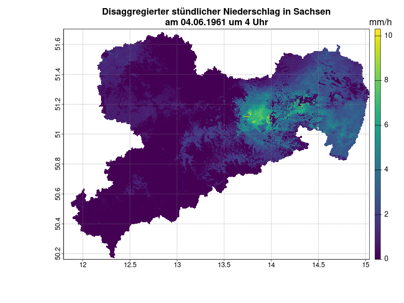
Hourly raster data on precipitation has only been available since the early 2000s thanks to radar measurements or the spatial interpolation of hourly station data. Thanks to specially developed methods, however, it is now possible to generate hourly precipitation grids from as early as 1951.
Why hourly precipitation grids?
Hourly precipitation grids offer numerous advantages:
- Spatial consistency: the high spatial resolution allows regional comparisons and a better assessment of local risks.
- Finer temporal resolution: They enable a detailed analysis of precipitation events, especially heavy rainfall, which would not be recognisable in daily values.
- Improved modelling: Hydrological and climatological models benefit from the precise input data, for example for flood forecasts or the assessment of extreme events.
- Seamless time series: They enable the investigation of trends and changes in precipitation behaviour over many decades.
Procedure
To create the hourly precipitation grids, the daily precipitation values are first disaggregated to hourly values using a model (gradient boosting). This involves relating measured hourly values of other meteorological variables available from 1951 onwards to the hourly precipitation.
In addition, a further model is used that learns the number of hours of precipitation per day as a function of the same predictors. Rasters of the meteorological variables are first calculated at hourly resolution for the desired time period. The methods and products described above are used here to generate the hourly precipitation grids. These grids serve as predictors for the application of the previously trained models.
The result is raster data with a spatial resolution of 100 metres and a temporal resolution of one hour – starting as early as 1951. This combination of high resolution and long time series is a novelty.
Quality and properties
The statistical properties of the original data, such as the distribution of precipitation over the day and the frequency of precipitation events, are largely retained. Spatial consistency is also guaranteed. In contrast to other methods, the actual events are better mapped. In addition, the data is climatologically consistent (spatially discrete annual total and trend).
The quality of the results is proven by a Heidke Skill Score of over 0.6 and a correlation in the range of 0.6 in the cross-validation – values that have not been achieved by any other method to date.
References
State Office for Environment, Agriculture and Geology (LfULG Saxony):
Spatial disaggregation of precipitation in ReKIS, gapless hourly grids for Saxony 1961-2023 (publication in preparation)
Fog and fog deposition
Description
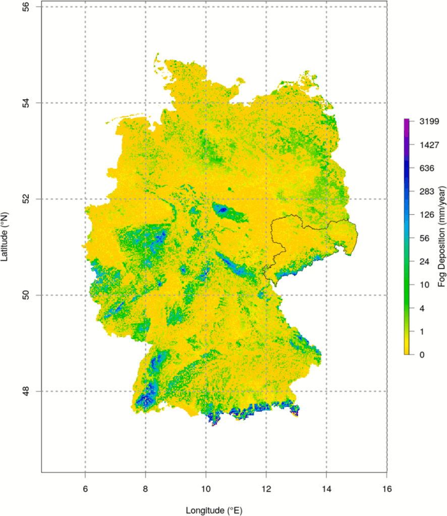
The calculation of fog and fog deposition determines the occurrence of fog on the ground and the deposition of fog droplets (fog deposition) from the atmosphere onto surfaces. In particular, the liquid water content (lwc) in the air near the ground is calculated and used as an indicator for the presence of fog. The product is based on meteorological measurement data such as temperature, relative humidity and terrain height, which are evaluated in hourly resolution in order to record the occurrence and intensity of fog spatially and temporally.
Why fog?
Monitoring fog and fog deposition is important for several reasons:
- Fog deposition can affect technical installations (e.g. wind turbines) and cause damage to vegetation, especially due to freezing fog
- Fog impairs visibility and poses a risk to road, air and shipping traffic.
- In certain ecosystems, such as cloud forests, fog is an important source of water and affects vegetation.
- Fog can be used as an alternative water resource, for example through fog collectors.
Procedure
The product provides information on when and where fog occurs and how much liquid water is contained in the air. Fog is defined as an accumulation of very small water droplets (diameter about 3-50 μm) in the atmosphere near the ground, which can reduce visibility to less than one kilometre. Fog deposition describes the deposition of these droplets on surfaces, which is relevant, for example, for the water balance of ecosystems or technical applications such as fog collectors. The key parameter is the liquid water content (lwc) per cubic metre of air, which is calculated from measurement data using physical models.
Quality and properties
The product is characterised by the following properties:
- Limitations of the measurement: Direct lwc measurements are rare and costly, which is why derived values (e.g. from visibility measurements) are often used. However, these derivations are subject to uncertainties and are site-specific
- Physically based calculation: Fog occurrence and fog deposition are determined on the basis of temperature, relative humidity and terrain height. The lwc is calculated with hourly resolution and spatial interpolation.
- Correction of measurement errors: As temperature and humidity measurements can be subject to errors (e.g. due to sensor ageing or calibration problems), correction procedures are used to improve data quality.
- Validation: The modelling results are compared with measurements of visibility and lwc at reference stations. The quality of fog detection is evaluated with skill scores (e.g. Heidke skill score) and shows a high agreement between model and observation.
- High temporal and spatial variability: Fog and its water content are highly variable, both temporally (e.g. between individual hours) and spatially (e.g. between different locations and altitudes).
References
State Office for Environment, Agriculture and Geology (LfULG Saxony):
Fog deposition Saony in ReKIS, daily raster data in 100 metre resolution for Saxony, 1961-2020
Literature
Körner, P., Kalaß, D., Kronenberg, R., Bernhofer, C., 2020. REAL-Fog: A simple approach for calculating the fog in the atmosphere at ground level. Meteorologische Zeitschrift. https://doi.org/10.1127/metz/2019/0976
Körner, P., Rico, K., Gliksman, D., Christian, B., 2021. REAL-Fog Part 2: A novel approach to calculate high resoluted spatio-temporal Fog Deposition: a daily fog deposition data set for entire Germany for 1949-2018. Journal of Hydrology 126360. https://doi.org/10.1016/j.jhydrol.2021.126360
Website
Daily updated hourly grids with validation:
Daily updated 10-minute grids: